Meet Vandra

April 13, 2026

5 Minutes read

Driving Operational Intelligence Through Point Anomaly Detection Using PELT

In today’s cloud-native enterprises, operational visibility is directly tied to business continuity. From infrastructure utilization and cloud cost patterns to ML model performance and API latency, organizations generate massive volumes of time-series data every second.

However, traditional monitoring approaches — largely based on static thresholds — struggle to adapt to evolving baselines. They often result in alert fatigue, delayed issue detection, or missed structural shifts in system behavior.

To enable intelligent, adaptive monitoring, organizations are increasingly adopting statistical change point detection techniques. One such efficient and scalable method is the PELT (Pruned Exact Linear Time) algorithm, implemented through the ruptures library.

This blog explores how enterprises can operationalize point anomaly detection using PELT and integrate it into modern data platforms for proactive decision-making.

Understanding Anomalies in Time-Series Data

Time-series anomalies typically fall into three categories:

Types of Anomalies in Time-Series Data

Time-series anomalies generally fall into three primary categories:

Point Anomaly

A point anomaly occurs when a single data point significantly deviates from the expected pattern.

Example: A sudden spike in CPU usage from 40% to 95% for one timestamp.

Common scenarios:

Infrastructure spikes
Sudden cost increase
Unexpected latency jump

Contextual Anomaly

A contextual anomaly occurs when a value is abnormal within a specific context but may appear normal globally.

Example: A temperature of 20°C might be normal during winter but anomalous during summer in a specific environment.

Common scenarios:

Seasonal demand spikes
Time-of-day usage patterns
Weekend vs weekday traffic

Collective Anomaly

A collective anomaly occurs when a sequence of data points together forms an abnormal pattern, even if individual points appear normal.

Example: A gradual increase in API latency over several minutes that collectively indicates system degradation.

This type is common in:

Infrastructure performance degradation
Network congestion
ML model drift patterns

Why Threshold-Based Detection Fails

Static alert rules, such as:

CPU exceeding 80%
Latency surpassing 300ms
DBU usage surpassing X

present significant limitations:

They require manual tuning.
They don’t adapt to evolving baselines.
They generate false positives during scale events.
They miss gradual structural shifts.

Instead of checking if a value crosses a line, change point detection identifies when the underlying distribution changes.

Change Point Detection: A Statistical Approach

Change point detection segments a time series into statistically homogeneous regions. It identifies points where:

The mean shifts
The variance changes
The distribution alters

One of the most efficient algorithms for this task is PELT (Pruned Exact Linear Time).

Understanding the PELT Algorithm

PELT (Pruned Exact Linear Time) is a change point detection algorithm designed to efficiently identify multiple structural changes within time-series data.

The core idea behind PELT is to partition a time series into segments such that each segment is statistically homogeneous.

It minimizes the following objective function:

Where:

C(segment) represents the cost function that measures how well the segment fits a statistical model.
m is the number of detected change points.
β (beta) is a penalty term that prevents detecting too many change points.

Why PELT is Efficient

Unlike many traditional algorithms with quadratic complexity, PELT uses dynamic programming and pruning techniques to remove unnecessary computations.

This results in near-linear time complexity, making it suitable for large enterprise datasets.

Implementation Using Python and Ruptures

The ruptures library provides a clean interface for multiple change point algorithms including PELT.

Implementation Walkthrough

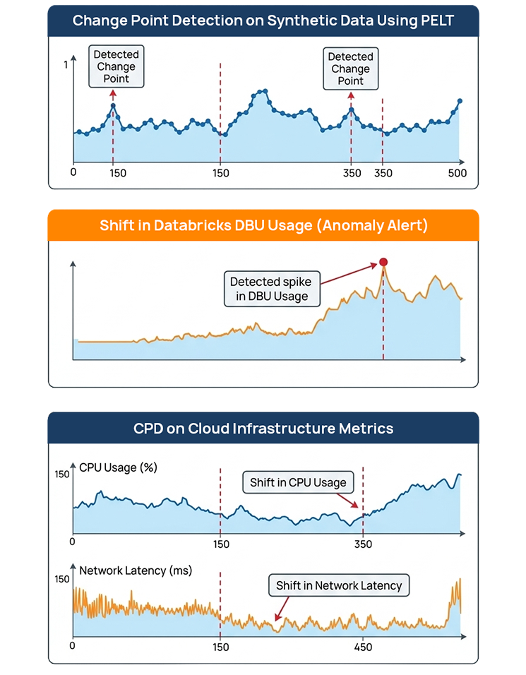
The following example demonstrates how to detect change points in a synthetic time-series dataset using the ruptures library.

The workflow consists of four key steps:

Generate a synthetic signal with multiple statistical segments.
Initialize the PELT algorithm using an appropriate cost model.
Predict change points using a penalty parameter.
Visualize the results to interpret the detected segments.

Example:

import numpy as np
import matplotlib.pyplot as plt
import ruptures as rpt

# Generate synthetic time-series data with distinct segments (structural shifts)
np.random.seed(42)
signal = np.concatenate([
np.random.normal(0, 1, 150), # Segment 1: Mean 0, Std Dev 1
np.random.normal(5, 1, 200), # Segment 2: Mean 5, Std Dev 1 (Shift in mean)
np.random.normal(2, 1, 150) # Segment 3: Mean 2, Std Dev 1 (Another shift)
])

# Initialize and fit the Pruned Exact Linear Time (PELT) change point detection algorithm
# using the L2 loss function (least squares)
algo = rpt.Pelt(model=”l2″).fit(signal)

# Predict the change points, using a penalty value (pen) of 10 to control the number of detected points
change_points = algo.predict(pen=10)

# Visualize the resulting signal and the detected change points
rpt.display(signal, change_points)
plt.title(“Change Point Detection on Synthetic Data using PELT”)
plt.show()

Choosing the Right Cost Model

The effectiveness of change point detection depends heavily on selecting the correct cost function.

The ruptures library supports several models:L2 Cost Model

Detects changes in mean while assuming constant variance.
Best suited for:
- Infrastructure metrics
- Cloud cost monitoring
- CPU utilization trends
- Latency spikes
Example use case: detecting sudden increases in cloud resource consumption.

RBF Cost Model

Detects changes in both mean and variance. Best suited for:
- Highly volatile signals
- Financial time-series data
- Sensor data streams
Example use case: detecting irregular patterns in IoT sensor readings.

Linear Cost Model

Detects changes in trends or slopes. Best suited for:
- Gradual performance degradation
- Long-term system drift
- Growth pattern analysis
Example use case: identifying slow increases in application response times.

Enterprise Use Case: Cloud Cost Monitoring

Consider a scenario where:

Databricks job costs spike unexpectedly
ETL runtime increases gradually
API latency baseline shifts

Rather than static alerts, we:

Collect metrics from monitoring systems.
Store them in a data lake (e.g., S3).
Run periodic anomaly detection jobs.
Trigger alerts only when structural shifts occur.

This reduces alert fatigue while improving operational intelligence.

Challenges and Considerations

Proper penalty tuning is essential.
Noisy signals may require smoothing.
Extremely high-frequency data may need preprocessing.
Real-time streaming detection requires additional orchestration.

Conclusion

Change point detection using the PELT algorithm offers a statistically grounded and computationally efficient solution for detecting structural shifts in time-series data. When operationalized correctly, it enables organizations to move from reactive monitoring to intelligent, adaptive anomaly detection.

By integrating libraries like ruptures into enterprise data pipelines, teams can build scalable and reliable anomaly detection systems that align with modern cloud-native architectures.